Marijuana Use and Depression In the United States
In this page, we utilize visualizing tools to explore the marijuana
use patterns across age groups and depression prevalence patterns in the
United States.
Age and Time-Since-Last-Marijuana-Use
In 2019 NSDUH, investigators collected information about time-since-last-marijuana-use. The question in the survey was: “how long has it been since you last used marijuana or hashish?” According to the code book, answers to this question are: “within the past 30 days (13.62%),”more than 30 days ago but within the last 12 months (7.47%)“,”more than 12 months ago (22.3%)“,”used in the past 30 days - logically assigned (0.01%), “used in the past 12 months - logically assigned (0.36%),”used at some point in the lifetime - logically assigned (0.39%), “never used marijuana (55.78%)”, “refused (0.03%)”, and “blank” (0.04%)“.
Additionally, we also want to use the age information which was
recoded as age2 in the 2019 NSDHU data set. Researchers
coded participants’ age into 17 categories, including:
- 1 = Respondent is 12 years old
- 2 = Respondent is 13 years old
- 3 = Respondent is 14 years old
- 4 = Respondent is 15 years old
- 5 = Respondent is 16 years old
- 6 = Respondent is 17 years old
- 7 = Respondent is 18 years old
- 8 = Respondent is 19 years old
- 9 = Respondent is 20 years old
- 10 = Respondent is 21 years old
- 11 = Respondent is 22-23 years old
- 12 = Respondent is 24-25 years old
- 13 = Respondent is 26-29 years old
- 14 = Respondent is 30-34 years old
- 15 = Respondent is 35-49 years old
- 16 = Respondent is 50-64 years old
- 17 = Respondent is 65+ years old
In our exploratory step, we excluded people who answered “never used marijuana” since they are not the group we are interested in. Then, we also dropped the logically assigned answers and people who answered “refused” and “blank” to avoid misclassification. Although this can reduce our statistical power, dropped values only count for less than 1% (0.83%) of the entire sample group. We assume dropping them will not affect the data presentation. Finally, we constructed two plots to explore the relationship between age and time-since-last-marijuana-use groups.
1. Age Distributions in Time-Since-Last-Marijuana-Use groups
mari_df %>%
  ggplot(aes(x = age2, y = mjrec, fill = factor(stat(quantile)))) +
  stat_density_ridges(geom = "density_ridges_gradient", calc_ecdf = TRUE, quantiles = 5, alpha = 0.5) +
  scale_fill_viridis_d(name = "Quintiles") +
  theme_ridges() +
  labs(x = "Age Categories",
       y = "Time-since-last-Marijuana-use",
       caption = "In Age categories: 1 = 12-yrs-old; 2 = 13-yrs-old; 3 = 14-yrs-old; 4 = 15-yrs-old; 5 = 16-yrs-old; 6 = 17-yrs-old; 7 = 18-yrs-old; 8 = 19-yrs-old; 9 = 20-yrs-old; \n10 = 21-yrs-old; 11 = 22-23 yrs-old; 12 = 24-25 yrs-old; 13 = 26-29 yrs-old; 14 = 30-34 yrs-old; 15 = 35-49 yrs-old; 16 = 50-64 yrs-old; 17 = >=65-yrs-old") +
  scale_x_continuous(breaks = c(1,2,3,4,5,6,7,8,9,10,11,12,13,14,15,16,17))+
  theme_minimal()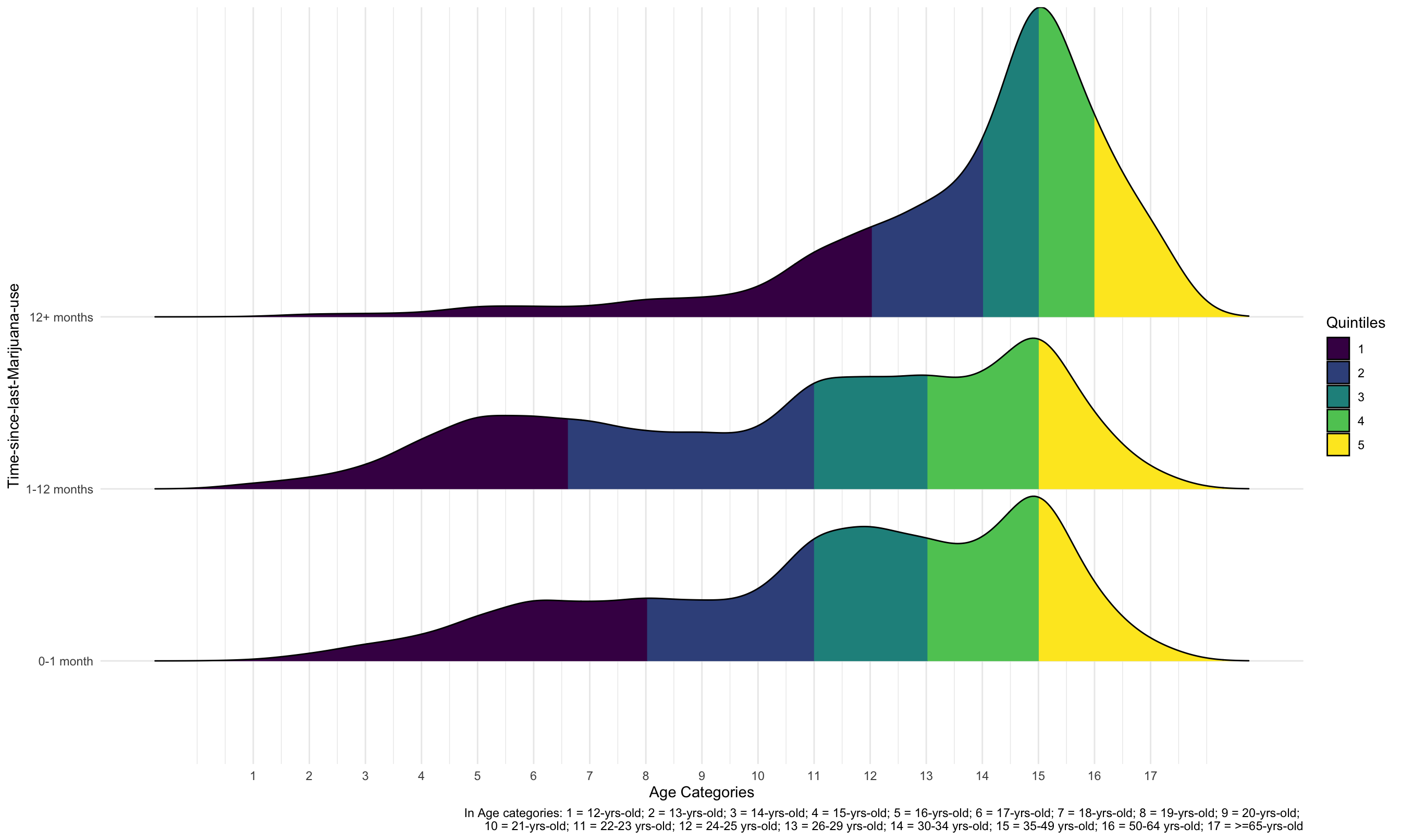
Comparing the age distributions among time-since-last-marijuana-use groups, only the curve for “12+ months” group has one obvious peak located at “age = 15” (35-49 yrs-old). Curves for other two groups look more like tri-modal distribution which has more than one peak.
If we compare quantiles among the 3 groups, the “12+ months” group has a very different age distribution. Younger than 34-year-olds contributed to the first two quintiles, while older than 50-year-olds contributed to the last quintile. However, the first two quintiles of the “0-1 month” and “1-12 months” groups were occupied by people younger than 23, and the last quintile by people older than 35. As a result, there are relatively more younger people in the “0-1 month” and “1-12 months” groups.
Additionally, the first 20% of people in the “0-1 month” group are people younger than 19, and the first 20% of people in the “1-12 months” group are people younger than 18 years old. This difference is relatively small, and these two groups have very similar age distribution based on quintiles.
2. Time-Since-Last-Marijuana-Use comparision Among Age Groups
mari_df %>%
  ggplot(aes(x = age2, fill = mjrec)) +
  geom_histogram(position = "dodge") +
  labs(x = "Age Categories",
       y = "Time-since-last-Marijuana-use",
       caption = "In Age categories: 1 = 12-yrs-old; 2 = 13-yrs-old; 3 = 14-yrs-old; 4 = 15-yrs-old; 5 = 16-yrs-old; 6 = 17-yrs-old; 7 = 18-yrs-old; 8 = 19-yrs-old; 9 = 20-yrs-old; \n10 = 21-yrs-old; 11 = 22-23 yrs-old; 12 = 24-25 yrs-old; 13 = 26-29 yrs-old; 14 = 30-34 yrs-old; 15 = 35-49 yrs-old; 16 = 50-64 yrs-old; 17 = >=65-yrs-old") +
  scale_x_continuous(breaks = c(1,2,3,4,5,6,7,8,9,10,11,12,13,14,15,16,17))+
  theme_minimal()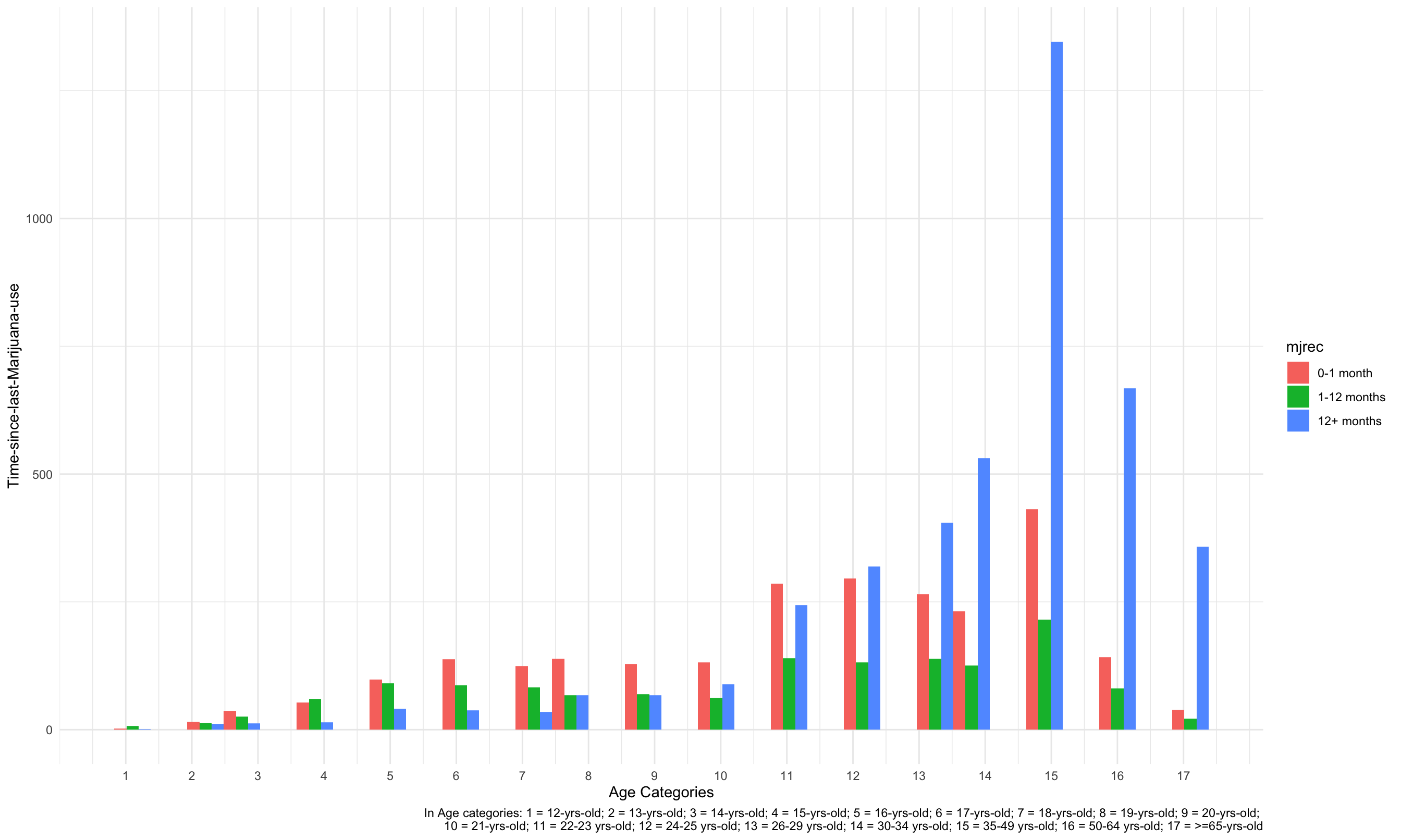
According to the histogram plot, in the 13-year-old, 14-year-old, 16-year-old, 17-year-old, 18-year-old, 19-year-old, 20-year-old, 21-year-old, 22-to-23-year-old groups, the time-since-last-marijuana-use for people are most likely be “0-1 month”. However, for people older than 24, the time-since-last-marijuana-use are more likely to be “12+ months”. Consequently, as people get older, they tend to use marijuana less often.
Marijuana Use In The Past 30 Days
In 2019 NSDUH, investigators collected information about #DAYS USED MARIJUANA PAST 30 DAYS. In this part, we excluded individuals who answered “ Don’t Know” “Refused” “Blank” “Legitimate Skip” to this question, which accounted for 14.32% of the total survey. The answers to this question were originally recorded as categories, including “1-2 days” “3-5 days” “6-9 days” “10-19 days” “20-29 days” “all 30 days”. In order to convert the variable to a continuous variable, we randomly assigned a number of days from its days range.
First, let’s explore the marijuana use pattern in the past 30 days of the survey in different age groups.
  graph_fendi %>%
    group_by(age_cat) %>%
    summarise(days = sum(days30)) %>%
knitr::kable(digits = 0)| age_cat | days |
|---|---|
| 12 - 15 | 101 |
| 16 - 19 | 481 |
| 20 - 25 | 285 |
| 26 - 29 | 44 |
| 30 - 34 | 30 |
| 35 - 49 | 70 |
| 50 - 64 | 33 |
| older_than_65 | 0 |
This table shows the cumulative numbers of days used marijuana in past 30 days in each age range. There were 56136 individuals participating the 2019 NSDUH survey. We can see that people who aged between 16 and 19 years accumulated the most number of days of marijuana using in the past 30 days of the survey, followed by those who aged between 20 and 25 years.
1. Number of Days Used Marijuana in Past 30 Days
graph_fendi %>%
    filter(days30 != 0) %>%
    ggplot(aes(x = age_cat, y = days30)) +
    geom_boxplot(aes(fill = age_cat), alpha = .5) +
  labs(x = "Age(years)", y = "Number of Days") +
  theme(plot.title = element_text(hjust = 0.5)) +
  theme_minimal()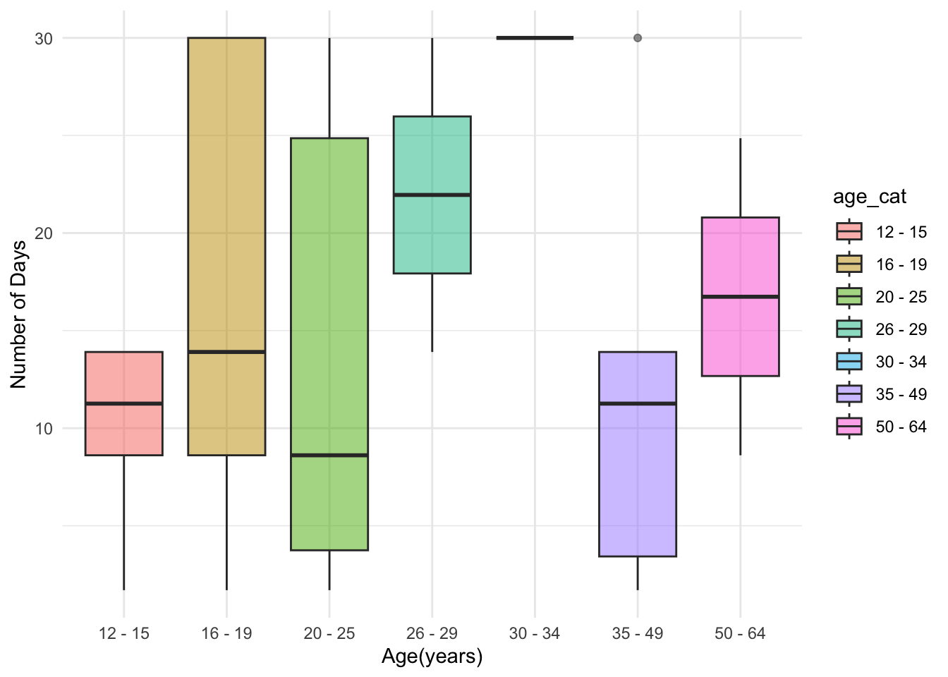
This graph shows the distribution of the numbers of days used marijuana in past 30 days of each individual. Those aged between 16 and 25 years had the widest range, while people who aged between 26 and 29 years had the highest mean for number of days used marijuana in past 30 days.
2. Percentage of Individuals Used Marijuana in Past 30 Days By Metro Area
Now, let’s take a look at the marijuana use pattern in the past 30 days of the survey in different types of metro areas.
graph_fendi %>%
  mutate(coutyp4 = as.character(coutyp4),
    coutyp4 = recode(coutyp4,
                     "1" = "Large Metro", "2" = "Small Metro", "3" = "Nonmetro"),
    coutyp4 = fct_relevel(coutyp4, "Large Metro", "Small Metro", "Nonmetro")) %>%
  group_by(coutyp4) %>%
    summarise( used30_percent = round(sum(use30)/n()*100, 2)) %>%
    ggplot(aes(x = coutyp4, y = used30_percent)) +
    geom_bar(stat = "identity", width = 0.5, fill = "steelblue") +
  geom_text(aes(label = used30_percent), vjust = 1.6, color = "white", size = 3.5) +
  labs(x = "Metro Area", y = "Percentage(%)") +
  theme(plot.title = element_text(hjust = 0.5)) +
  theme_minimal()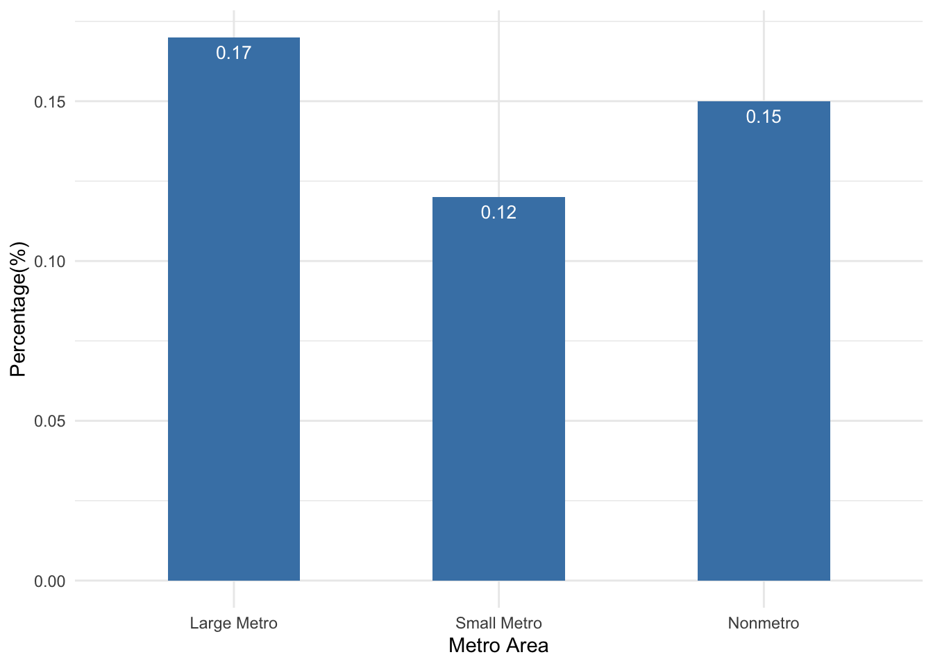
We can see that the marijuana use patterns in the past 30 days did not vary much across different metro areas. Slightly more individuals from the “large Metro” area (0.17%) used marijuana in the past 30 days of the survey than the other two types of metro areas.
Age When People First Started Using Marijuana
info_scatterplot = info_scatter %>%
  filter(irmjage != 991) %>%
  group_by(irmjage) %>%
  summarise(number_people = n()) %>%
  ggplot(aes(x = irmjage, y = number_people)) +
  geom_point() +
  geom_smooth() +
  labs(x = "Age of first used marijuana", y = "Frequency(number of people)",
       title = "Age When First Used among people who used MARIJUANA/HASHISH") +
  theme_minimal()


info_scatterplot 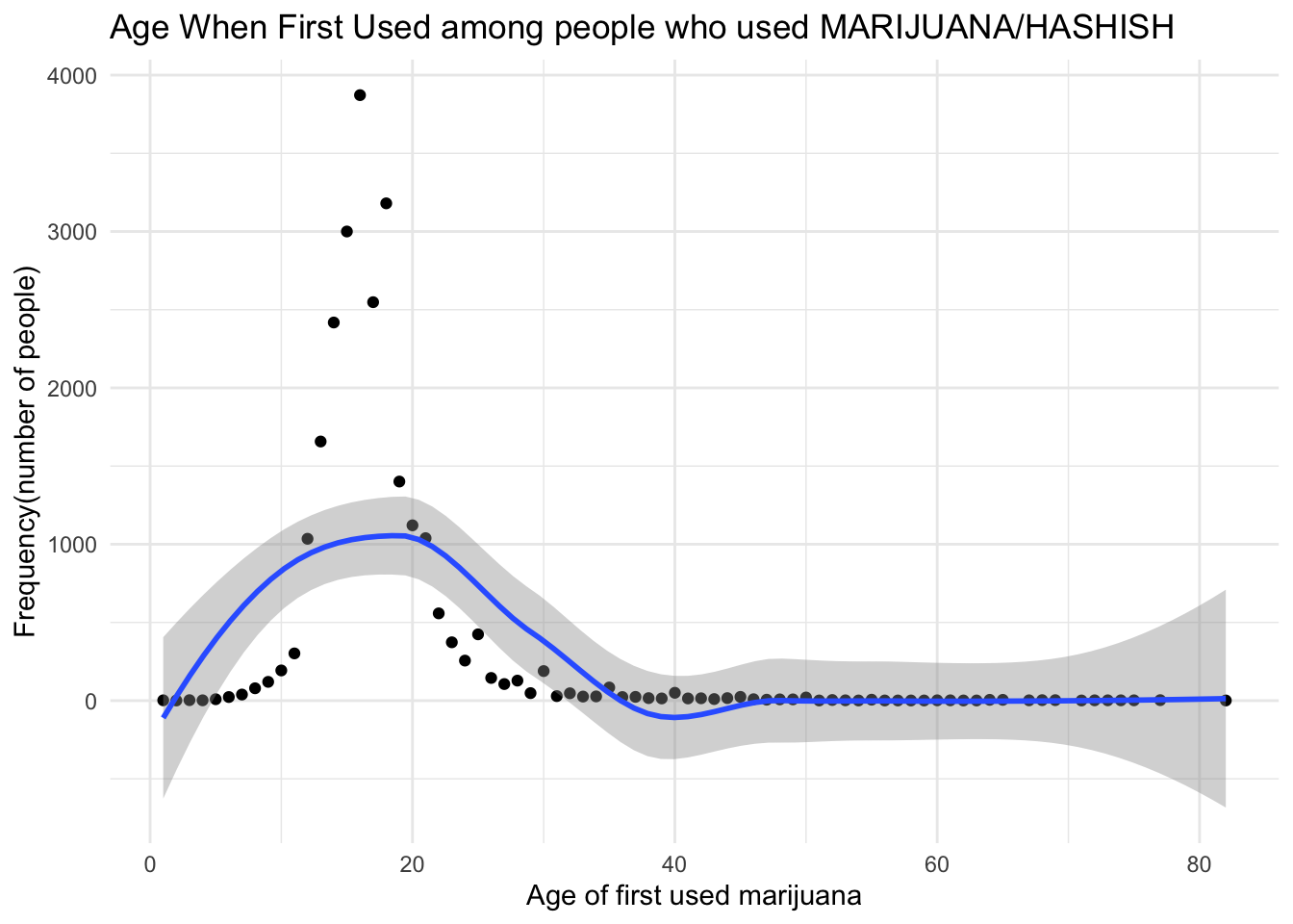
In this part, we created a scatter plot to show the age when first used MARIJUANA/HASHISH and frequency of people in each year. We excluded people who never use MARIJUANA/HASHISH in this plot. Because, without doubts, most people never use MARIJUANA/HASHISH. In our dataset, there are 31340 people who never use MARIJUANA/HASHISH. Therefore, after excluding people who never use MARIJUANA/HASHISH, it is more clear to see the distribution of Age when First Used among people who used MARIJUANA/HASHISH.
From this plot, we could conclude that most people who used Marijuana started between 10 and 30 years old when first used marijuana. So, it is necessary to focus on youth population during our further steps.
Depression Prevalence Pattern
Now, we have finished exploring the marijuana use pattern in the United States. In this last part, we would like to show the prevalence of depression in the United States and how the prevalence varies across different geographic areas among youths and adults. The association between marijuana use and depression is explored under the tab Statistical Analysis.
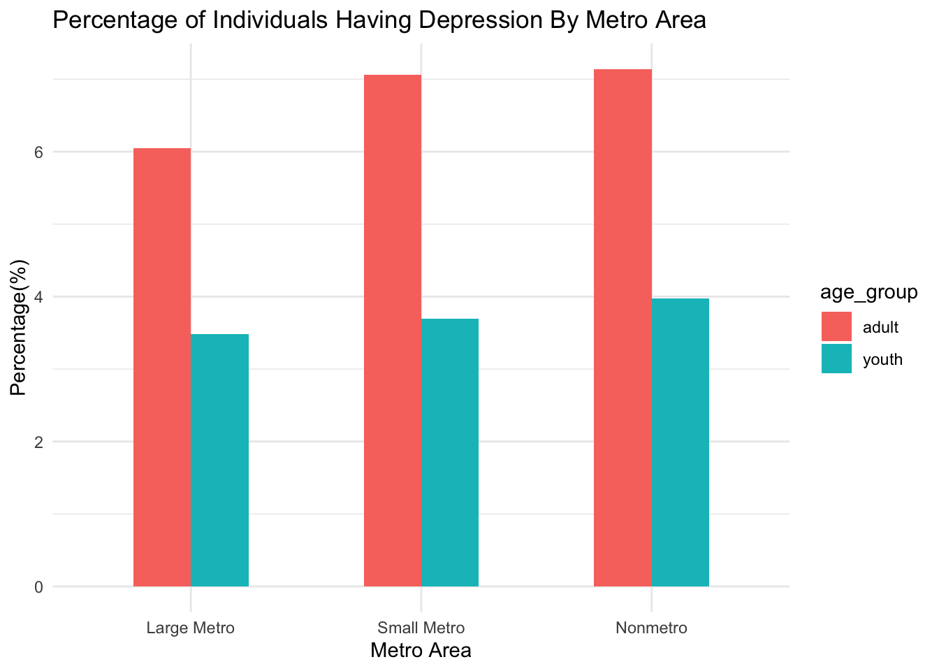
Looking at the graph below,we can see that depression is more prevalent among adults than youth across all three metro areas. Regardless of the age group, depression is more prevalent in the non-metro and the small-metro area than the large-metro area.
graph_fendi %>%
  mutate(coutyp4 = as.character(coutyp4),
    coutyp4 = recode(coutyp4,
                     "1" = "Large Metro", "2" = "Small Metro", "3" = "Nonmetro"),
    coutyp4 = fct_relevel(coutyp4, "Large Metro", "Small Metro", "Nonmetro")) %>%
  group_by(coutyp4) %>%
    summarise( youth = round(sum(youth_dpr, na.rm=TRUE)/n()*100, 2),
               adult = round(sum(adult_dpr, na.rm=TRUE)/n()*100, 2)) %>%
  pivot_longer(
    youth:adult,
    names_to = "age_group",
    values_to = "dpr_percent"
  ) %>%
  ggplot(aes(x = coutyp4, y = dpr_percent, fill = age_group)) +
    geom_bar(stat = "identity", width = 0.5, position = "dodge") +
    labs(title = "Percentage of Individuals Having Depression By Metro Area",
         x = "Metro Area", y = "Percentage(%)") +
    theme(plot.title = element_text(hjust = 0.5)) +
    theme_minimal()